This article discusses how we estimate the population variance of a normal distribution, often denoted as $\sigma^2$. Typically, we use the sample variance estimator defined as:
\begin{equation}s^{2}=\frac{1}{n-1} \sum_{i=1}^{n}\left(x_{i}-\bar{x}\right)^{2}\end{equation}
Here, $\bar{x}=\frac{\sum_{i=1}^{n} x_{i}}{n}$ denotes sample mean. However, it’s not intuitively clear why we divide the sum of squares by $(n - 1)$ instead of $n$, where $n$ stands for sample size, to get the sample variance. In statistics, this is often referred to as Bessel’s correction.
Another feasible estimator is obtained by dividing the sum of squares by sample size, and it is the maximum likelihood estimator (MLE) of the population variance:
\begin{equation}\hat{\sigma}^{2}=\frac{1}{n} \sum_{i=1}^{n}\left(x_{i}-\bar{x}\right)^{2}\end{equation}
Which one is better?
By applying the Bias-variance decomposition and Cochran’s theorem, this article attempts to address these questions. It concludes that:
- We use $(n - 1)$ in the sample variance estimator because we want to obtain an unbiased estimator of the population variance.
- Dividing the sum of squares by $n$ still gives us a good estimator as it has a lower mean squared error (MSE).
We will also go over an experiment implemented in Python to verify our conclusions numerically. Stay tuned!
Suppose we have a sample $X_{n\times p}=\begin{bmatrix}x_1, x_2, \dots, x_p\end{bmatrix}$, where $x_i \stackrel{iid}{\sim} N(\mu, \sigma^2)$. We are considering two estimators of the population variance $\sigma^2$: the sample variance estimator and the MLE estimator.
Evaluating Estimators: Bias, Variance, and MSE
We will first introduce some metrics to evaluate these estimators, namely, bias, variance, and MSE. Assuming we are estimating population parameter $\theta$ and our estimator $\hat{\theta}$ is a function of data: $\hat{\theta}=\hat{\theta}\left(X\right)_{p\times 1}$, and error term $\epsilon\left(\hat{\theta}\right):=\hat{\theta}-\theta$. Then we can define:
\begin{equation}\begin{aligned} \operatorname{MSE}(\hat{\theta})&:=\mathbb{E}[\epsilon^T \epsilon]=\mathbb{E}[\sum_{i=1}^p (\hat{\theta_i}-\theta_i)^2] \\ \operatorname{Bias}(\hat{\theta})&:=\left\Vert\mathbb{E}[\hat{\theta}]-\theta\right\Vert \\ \operatorname{Variance}(\hat{\theta})&:=\mathbb{E}\left[\left\Vert\hat{\theta}-\mathbb{E}[\hat{\theta}]\right\Vert_{2}^{2}\right] \end{aligned}\end{equation}
Intuitively, bias measures how our estimates diverge from the underlying parameter. Since our estimates change with data, variance measures the expectation of them diverging from their averages across different data sets. MSE is a comprehensive measure and can be decomposed into $(\text{Bias}^2 + \text{Variance})$ as follows.
\begin{equation}\begin{aligned} \text { Bias }^{2}+\text { variance } &=|\mathbb{E}[\hat{\theta}]-\theta|^{2}+\mathbb{E}\left[|\hat{\theta}-\mathbb{E}[\hat{\theta}]|^{2}\right] \\ &=\mathbb{E}[\widehat{\theta}]^{\top} \mathbb{E}[\hat{\theta}]-2 \theta^{\top} \mathbb{E}[\hat{\theta}]+\theta^{\top} \theta+\mathbb{E}\left[\hat{\theta}^{\top} \hat{\theta}-2 \widehat{\theta}^{\top} \mathbb{E}[\widehat{\theta}]+\mathbb{E}[\hat{\theta}]^{\top} \mathbb{E}[\widehat{\theta}]\right] \\ &=\mathbb{E}[\widehat{\theta}]^{\top} \mathbb{E}[\widehat{\theta}]-2 \theta^{\top} \mathbb{E}[\hat{\theta}]+\theta^{\top} \theta+\mathbb{E}\left[\widehat{\theta}^{\top} \hat{\theta}\right]-\mathbb{E}[\hat{\theta}]^{\top} \mathbb{E}[\widehat{\theta}] \\ &=-2 \theta^{\top} \mathbb{E}[\hat{\theta}]+\theta^{\top} \theta+\mathbb{E}\left[\hat{\theta}^{\top} \widehat{\theta}\right] \\ &=\mathbb{E}\left[-2 \theta^{\top} \hat{\theta}+\theta^{\top} \theta+\widehat{\theta}^{\top} \hat{\theta}\right] \\ &=\mathbb{E}[\left\Vert\theta-\hat{\theta}\right\Vert^{2}]=\operatorname{MSE}[\hat{\theta}] \end{aligned}\end{equation}
In the following sections, we will apply Cochran’s theorem to derive the bias and variance of our two estimators and make a comparison.
Sample Variance Estimator
Cochran’s theorem is often used to justify the probability distributions of statistics used in the analysis of variance (ANOVA). We will skip the proof and simply apply it to our case.
Cochran’s theorem shows that the sum of squares of a set of $iid$ random variables that are generated from standard normal has a chi-squared distribution with $(n - 1)$ degrees of freedom. In other words, $\frac{(n-1) s^{2}}{\sigma^{2}}=\sum_{i=1}^{n}\left(\frac{x_{i}-\bar{x}}{\sigma}\right)^{2} {\sim} \chi_{n-1}^{2}$, where $\frac{x_{i}-\bar{x}}{\sigma} \stackrel{iid}{\sim} N(0, 1)$. Therefore $\mathbb{E}\left[\frac{(n-1) s^{2}}{\sigma^{2}}\right]=\mathbb{E}\left[\chi_{n-1}^{2}\right]=n-1$ and $\mathbb{E}\left[s^{2}\right]=\sigma^{2}$. We have:
\begin{equation}\operatorname{Bias}\left[s^{2}\right]=0\end{equation}
From this, we see that sample variance estimator is desirably an unbiased estimator of the population variance. We can then write out its variance and MSE. It’s clear that $\operatorname{Var}\left(\frac{(n-1) s^{2}}{\sigma^{2}}\right)=\operatorname{Var}\left(\chi_{n-1}^{2}\right)=2(n-1)$. We have:
\begin{equation}\begin{aligned} \operatorname{Var}\left[s^{2}\right]&=\frac{2 \sigma^{4}}{n-1} \\ \operatorname{MSE}\left[s^{2}\right]&=\frac{2 \sigma^{4}}{n-1} \end{aligned}\end{equation}
MLE Estimator
In the same manner, we can derive the bias, variance, and MSE for the MLE estimator of population variance. It’s not hard to see that $\mathbb{E}\left[\frac{n \hat{\sigma}^{2}}{\sigma^{2}}\right]=\mathbb{E}\left[\chi_{n-1}^{2}\right]=n-1$, and $\mathbb{E}\left[\hat{\sigma}^{2}\right]=\frac{(n-1) \sigma^{2}}{n}$. Therefore:
\begin{equation}\operatorname{Bias}\left[\hat{\sigma}^{2}\right]=-\frac{1}{n} \sigma^{2}\end{equation}
From this, we know why we typically divide the sum of squares by $(n - 1)$ to calculate sample variance. The MLE estimator is a biased estimator of the population variance and it introduces a downward bias (underestimating the parameter). The size of the bias is proportional to population variance, and it will decrease as the sample size gets larger.
In terms of variance, $\operatorname{Var}\left(\frac{n \hat{\sigma}^{2}}{\sigma^{2}}\right)=\operatorname{Var}\left(\chi_{n-1}^{2}\right)=2(n-1)$. We have:
\begin{equation}\begin{aligned} \operatorname{Var}\left[\hat{\sigma}^{2}\right]&=\frac{2 \sigma^{4}(n-1)}{n^{2}} \\ \operatorname{Var}\left[s^{2}\right]-\operatorname{Var} \left[\hat{\sigma}^{2}\right]&=\frac{2 \sigma^{4}(2 n-1)}{n^{2}(n-1)}>0 \end{aligned}\end{equation}
We find that the MLE estimator has a smaller variance. The size of the gap is proportional to population variance. Further, $\frac{\partial\left[\operatorname{Var}\left(s^{2}\right)-\operatorname{Var}\left(\hat{\sigma}^{2}\right)\right]}{\partial n}=-\frac{2 \sigma^{4}\left(4 n^{2}-5 n+2\right)}{(n-1)^{2} n^{3}}<0$. We can see that MLE estimator’s advantage on variance over the sample variance estimator decreases as the sample size gets larger. In terms of the MSE:
\begin{equation}\begin{aligned} \operatorname{MSE}\left[\hat{\sigma}^{2} \right]&=\left(-\frac{\sigma^{2}}{n}\right)^{2}+\frac{2 \sigma^{4}(n-1)}{n^{2}}=\frac{\sigma^{4}(2 n-1)}{n^{2}} \\ \operatorname{MSE}\left[\hat{s}^{2} \right]- \operatorname{MSE}\left[\hat{\sigma}^{2} \right]&=\frac{2 \sigma^{4}}{n(n-1)}>0 \end{aligned}\end{equation}
We find that the MLE estimator also has a smaller MSE. As expected, the size of the gap is proportional to population variance and decreases as the sample size gets larger.
Numerical Experiment
In this section, we will verify our conclusions derived above. We will generate 100,000 samples $iid$ of size $n$ from $N(0, \sigma^2)$. $X$ is of shape $n × 100000$, with each column vector representing one sample of shape $n × 1$.
We will start with $n = 10$ and $\sigma^2 = 1$. The codes below help generate data and evaluate the estimators. Note the use of argument ddof as it specifies what to subtract from sample size for that estimator.
Evaluate the sample variance estimator:
1
2
3
print(to_print.format("Sample variance estimator", *evaluateVarEstimator(X)))

# Sample variance estimator: Bias = 0.0001, Variance = 0.2225, MSE = 0.2225.
Now the MLE:
1
2
3
print(to_print.format("Sample variance estimator", *evaluateVarEstimator(X, ddof=0)))

# MLE estimator: Bias = -0.0999, Variance = 0.1802, MSE = 0.1902.
As expected, the MLE estimator introduces a downward bias while that of the sample variance estimator is negligible. Meanwhile, the MLE estimator has lower variance and MSE.
We will change our configuration of sample size and population variance to see what happens to the gap in bias, variance, and MSE between the sample variance estimator and the MLE estimator:
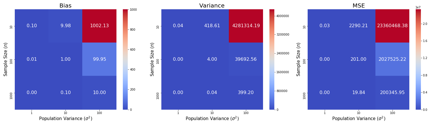
As expected, the gaps in bias, variance, and MSE between the sample variance estimator and the MLE estimator increase as population variances increases and decrease drastically as sample size increases. Check the codes that I used to generate the visualizations:
This blog was originally published on @Medium with @Towards Data Science at this link.
Background picture source: Krzysztof_War on Pixabay