该回答写在知乎问题为什么样本方差(sample variance)的分母是 n-1?下,现搬运到此。内容与我的英文博客:Estimate Population Variance: should we divide by n - 1 or n 大致相同。
问题下已经有许多非常精彩的回答了。在估计总体方差时,比较常用的估计量(estimator)包括样本方差估计量 $s^{2}=\frac{1}{n-1} \sum_{i=1}^{n}\left(x_{i}-\bar{x}\right)^{2}$和其最大似然估计量(maximum likelihood estimator, MLE)$\hat{\sigma}^{2}=\frac{1}{n} \sum_{i=1}^{n}\left(x_{i}-\bar{x}\right)^{2}$。
作为一个机器学习爱好者,我来从偏差-方差权衡(bias–variance tradeoff)的角度,结合Cochran定理比较一下二者的特性。先放上结论:
- 样本方差估计量的分母是 $n-1$的主要原因是我们希望获得一个总体方差的无偏估计量(unbiased estimator),这一点在许多回答中都已经被提及
- 总体方差的最大似然估计量有更低的方差(variance)和均方误差(mean square error,MSE),因而在一些场景中也适用
下文中,我们将首先回顾一下偏差-方差权衡,并介绍估计量的三个评价指标,偏差(bias)、方差、以及均方误差。
偏差-方差权衡
首先回顾一下偏差-方差权衡。当我们以估计量 $\hat{\theta}$估计总体参数 $\theta$时,估计偏误$\epsilon\left(\hat{\theta}\right)$可以表示为$\hat{\theta}-\theta$。作为衡量和比较估计量表现的评价指标,直观地讲,偏差衡量了估计值与总体参数的差距;而因为估计值是样本数据的函数,方差衡量了估计值在不同样本上与其平均值的离散程度。定义如下:
\begin{equation}\begin{aligned} \operatorname{MSE}(\hat{\theta})&:=\mathbb{E}[\epsilon^T \epsilon]=\mathbb{E}[\sum_{i=1}^p (\hat{\theta_i}-\theta_i)^2] \\ \operatorname{Bias}(\hat{\theta})&:=\left\Vert\mathbb{E}[\hat{\theta}]-\theta\right\Vert \\ \operatorname{Variance}(\hat{\theta})&:=\mathbb{E}\left[\left\Vert\hat{\theta}-\mathbb{E}[\hat{\theta}]\right\Vert_{2}^{2}\right] \end{aligned}\end{equation}
按照如下步骤,我们可以将均方误差分解为$(\text{bias}^2 + \text{variance})$:
\begin{equation}\begin{aligned} \text { Bias }^{2}+\text { variance } &=|\mathbb{E}[\hat{\theta}]-\theta|^{2}+\mathbb{E}\left[|\hat{\theta}-\mathbb{E}[\hat{\theta}]|^{2}\right] \\ &=\mathbb{E}[\widehat{\theta}]^{\top} \mathbb{E}[\hat{\theta}]-2 \theta^{\top} \mathbb{E}[\hat{\theta}]+\theta^{\top} \theta+\mathbb{E}\left[\hat{\theta}^{\top} \hat{\theta}-2 \widehat{\theta}^{\top} \mathbb{E}[\widehat{\theta}]+\mathbb{E}[\hat{\theta}]^{\top} \mathbb{E}[\widehat{\theta}]\right] \\ &=\mathbb{E}[\widehat{\theta}]^{\top} \mathbb{E}[\widehat{\theta}]-2 \theta^{\top} \mathbb{E}[\hat{\theta}]+\theta^{\top} \theta+\mathbb{E}\left[\widehat{\theta}^{\top} \hat{\theta}\right]-\mathbb{E}[\hat{\theta}]^{\top} \mathbb{E}[\widehat{\theta}] \\ &=-2 \theta^{\top} \mathbb{E}[\hat{\theta}]+\theta^{\top} \theta+\mathbb{E}\left[\hat{\theta}^{\top} \widehat{\theta}\right] \\ &=\mathbb{E}\left[-2 \theta^{\top} \hat{\theta}+\theta^{\top} \theta+\widehat{\theta}^{\top} \hat{\theta}\right] \\ &=\mathbb{E}[\left\Vert\theta-\hat{\theta}\right\Vert^{2}]=\operatorname{MSE}[\hat{\theta}] \end{aligned}\end{equation}
不难看出,均方误差是综合了偏差和方差的评价指标。
下面一节中,我们将运用Cochran定理分别计算样本估计量和总体方差的最大似然估计量的偏差、方差和均方误差并作比较。
评估样本方差估计量
Cochran定理的证明与回答的关系不大,此处略去。
其表明,一系列产生于标准正态分布且独立同分布($\overset{iid}{\sim}N(0,1)$)的随机变量的平方和服从自由度为$(n-1)$ 的卡方分布(chi-square distribution)。
将结论用于分析样本方差估计量,不难看出$\frac{(n-1) s^{2}}{\sigma^{2}}=\sum_{i=1}^{n}\left(\frac{x_{i}-\bar{x}}{\sigma}\right)^{2} {\sim} \chi_{n-1}^{2}$。其中,$\frac{x_{i}-\bar{x}}{\sigma} \stackrel{iid}{\sim} N(0, 1) $。因此,$\mathbb{E}\left[\frac{(n-1) s^{2}}{\sigma^{2}}\right]=\mathbb{E}\left[\chi_{n-1}^{2}\right]=n-1$,即$\mathbb{E}\left[s^{2}\right]=\sigma^{2}$。也就是说:
\begin{equation}\begin{aligned}\operatorname{Bias}\left[s^{2}\right]&=\mathbb{E}\left[s^{2}\right]-\sigma^{2}=\sigma^{2}-\sigma^{2}\\&=0\end{aligned}\end{equation}
由此,样本方差估计量是总体方差的无偏估计量。
再看样本方差估计量的方差,$\operatorname{Var}\left(\frac{(n-1) s^{2}}{\sigma^{2}}\right)=\operatorname{Var}\left(\chi_{n-1}^{2}\right)=2(n-1)$。因此:
\begin{equation}\begin{aligned} \operatorname{Var}\left[s^{2}\right]&=\frac{2 \sigma^{4}}{n-1} \\ \operatorname{MSE}\left[s^{2}\right]&=\frac{2 \sigma^{4}}{n-1} \end{aligned}\end{equation}
类似地,将结论用于分析总体方差的最大似然估计量,不难看出$\mathbb{E}\left[\frac{n \hat{\sigma}^{2}}{\sigma^{2}}\right]=\mathbb{E}\left[\chi_{n-1}^{2}\right]=n-1$。因此:
\begin{equation}\begin{aligned}\operatorname{Bias}\left[\hat{\sigma}^{2}\right]&=\mathbb{E}\left[\hat{\sigma}^{2}\right]-\sigma^{2}=\frac{(n-1) \sigma^{2}}{n}-\sigma^{2}\\&=-\frac{1}{n} \sigma^{2}\le0 \end{aligned}\end{equation}
也就是说,总体方差的最大似然估计量是总体方差的有偏估计量,并且倾向于低估总体方差。再看其方差和均方误差。 $\operatorname{Var}\left(\frac{n \hat{\sigma}^{2}}{\sigma^{2}}\right)=\operatorname{Var}\left(\chi_{n-1}^{2}\right)=2(n-1)$,因此:
\begin{equation}\begin{aligned} \operatorname{Var}\left[\hat{\sigma}^{2}\right]&=\frac{2 \sigma^{4}(n-1)}{n^{2}} \\ \operatorname{MSE}\left[\hat{\sigma}^{2} \right]&=\left(-\frac{\sigma^{2}}{n}\right)^{2}+\frac{2 \sigma^{4}(n-1)}{n^{2}}\\&=\frac{\sigma^{4}(2 n-1)}{n^{2}} \end{aligned}\end{equation}
最后,我们以偏差、方差和均方误差作为评价标准,比较一下总体方差的样本方差估计量和最大似然估计量:
- 如果以偏差作为评价标准:很直观地,样本方差估计量是总体方差的无偏估计量,总体方差的最大似然估计量会引入向下偏差,偏差的绝对值大小与总体方差参数成正比关系,与样本量成反比关系。样本方差估计量(分母为 $n-1$ )更好。
- 如果以方差作为评价标准:由$\operatorname{Var}\left[s^{2}\right]-\operatorname{Var} \left[\hat{\sigma}^{2}\right]=\frac{2 \sigma^{4}(2 n-1)}{n^{2}(n-1)}>0$可知最大似然估计量的方差更小,而且二者方差的差距与总体方差参数成正比关系,与样本量成反比关系。总体方差的最大似然估计量(分母为$n$)更好。
- 如果以均方误差作为评价标准:由$\operatorname{MSE}\left[\hat{s}^{2} \right]- \operatorname{MSE}\left[\hat{\sigma}^{2} \right]=\frac{2 \sigma^{4}}{n(n-1)}>0$,可知最大似然估计量的均方误差更小,而且这一差距与总体方差参数成正比关系,与样本量成反比关系。总体方差的最大似然估计量更好。
下面一节,将以数值实验的形式验证上面三条结论。
数值实验
首先,按照 $\overset{iid}{\sim}N(0, \sigma^2)$生成一个样本量为100000,样本容量为 $n$的数据矩阵$X$ 。换句话说,$X$中的每一个列向量$X_{i, n\times 1}\overset{iid}{\sim}N(0, \sigma^2)$代表一个大小为$n$样本。我们可以尝试$n=10, \sigma^2=1$:
1
2
3
4
5
6
7
8
9
10
11
12
import numpy as np


np.random.seed(123)
LOC = 0
N = 100000

# Generate data
n = 10
sigma2 = 1

X = np.random.normal(LOC, sigma2, size=(n, N))
我们可以用下面的evaluate_var_estimator函数来计算总体方差的样本方差估计量和最大似然估计量的偏差,方差和均方误差:
1
2
3
4
5
6
7
8
9
10
11
12
13
14
15
16
def evaluateVarEstimator(X, ddof=1):
    est = X.var(axis=0, ddof=ddof)
    bias = est.mean() - sigma2
    var = est.var()

    return bias, var, bias ** 2 + var


to_print = ("{}: Bias = {:.4f}, Variance = {:.4f}"
            ", MSE = {:.4f}.")

print(to_print.format("Sample variance estimator", *evaluateVarEstimator(X)))
# Output: Sample variance estimator: Bias = 0.0001, Variance = 0.2225, MSE = 0.2225.

print(to_print.format("Sample variance estimator", *evaluateVarEstimator(X, ddof=0)))
# Output: MLE estimator: Bias = -0.0999, Variance = 0.1802, MSE = 0.1902.
与前面一节的结论相同地,样本方差估计量是总体方差的无偏估计量,而其最大似然估计量引入了向下偏差。与此同时,后者有更小的方差和均方误差。
下面,我们可以通过改变样本量$n$和总体方差参数 $\sigma^2$ 观察两个估计量偏差、方差和均方误差的差值的变化情况。使用如下代码简单验证:
1
2
3
4
5
6
7
8
9
10
11
12
13
ns = [10, 100, 1000]
sigma2s = [1, 10, 100]

gaps = np.zeros(shape=(3, len(ns), len(sigma2s)))

for i in range(len(ns)):
    for j in range(len(sigma2s)):
        X = np.random.normal(LOC, sigma2s[j], size=(ns[i], N))
        gap = np.array(evaluateVarEstimator(X)) -\
              np.array(evaluateVarEstimator(X, ddof=0))

        for l, metric in enumerate(gap):
            gaps[l, i, j] = metric
并且使用热力图(heatmap)可视化结果(每一个方格代表差值的大小):
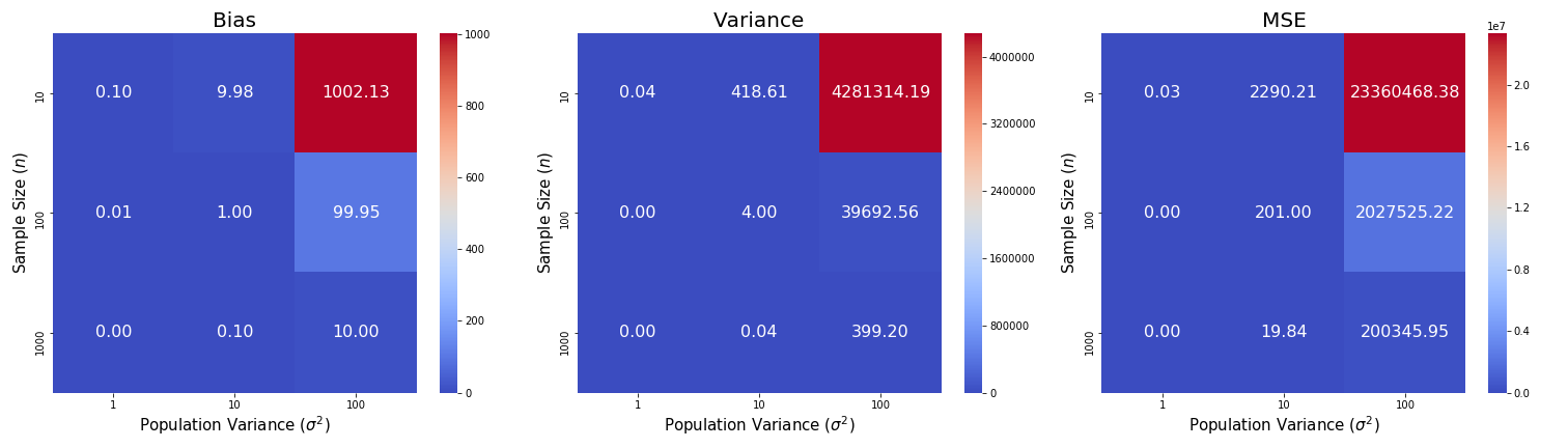
正如预期,偏差、方差和均方误差的差值随样本量$n$的增加而减小,随总体方差$\sigma^2$的增加而增加。
感谢阅读。最后,附上知乎回答链接:为什么样本方差(sample variance)的分母是 n-1? - 知乎
Background picture source: valentin hintikka on Pixabay