This article discusses what is principal component analysis (PCA), how we do it using eigenvalue decomposition (EVD) or singular value decomposition (SVD), and why the SVD implementation is better.
Principal Component Analysis
Intuitively, PCA is a transformation procedure that converts a data matrix with possibly correlated features into a set of linearly uncorrelated variables called principal components. Each principal component is a linear combination of the original features ($\text{PC}_i=X\phi_i$, here $\text{PC}_i$ denotes the $i^{\text{th}}$ principal component and $\phi_i$ stands for the weights) and accounts for the largest possible variance while being orthogonal to the preceding components (if $i\neq j$, $\langle\text{PC}_i, \text{PC}_j\rangle=0$).
Given a feature matrix $X$ of shape $n \times p$ that is centered, i.e. column means have been subtracted and are now equal to zero, typical use cases of PCA include:
- Dimensionality reduction: find a lower-dimensional approximation of $X$ of shape $n × k$ (where $k$ is much smaller than $p$) while maintaining most of the variances, as a preprocessing step for classification or visualization.
- Feature engineering: create a new representation of $X$ with $p$ linearly uncorrelated features.
- Unsupervised learning: extract $k$ principal components (where $k$ is often much smaller than $p$). Understand the dataset by looking at how are the original features contributing to these factors.
Conceptually, it’s important to keep in mind that PCA is an approach of multivariate data analysis and both EVD and SVD are numerical methods.
PCA through Eigenvalue Decomposition
Conventionally, PCA is based on the EVD on the sample covariance matrix $C$. Assuming that $X$ is centered, we know that $C=\frac{\Sigma_{i=1}^{n} x_{i} x_{j}^{T}}{n-1}=\frac{X^{T} X}{n-1}$. $C$ is of shape $p \times p$. It is symmetric and hence always diagonalizable. We can apply eigenvalue decomposition:
\begin{equation}C=Q_{p \times p} \Lambda_{p \times p} Q^{T}\end{equation}
$Q$ is an orthogonal matrix ($Q^TQ=QQ^T=I$) and its columns are the eigenvectors of $C$ ($Q=\begin{bmatrix}q_1, q_2, \dots, q_p\end{bmatrix}$, $Cq_i=\sigma_iq_i$). $q_i$ denotes the $i^{\text{th}}$ column of $Q$ is also called the $i^{\text{th}}$ principal direction. $\Lambda$ is a diagonal matrix with eigenvalues in the decreasing order on the diagonal ($\sigma_1\ge \sigma_2 \ge \dots \ge \sigma_p > 0$).
Principal components are the projections of the original feature matrix on the principal directions and can be obtained with $XQ$. The proportion of total variance that the $i^{\text{th}}$ principal component explains is $\frac{\sigma_i}{\sum_{i=1}^{i=p}\sigma_i}$.
Below is an implementation of PCA through EVD in Python:
PCA through Singular Value Decomposition
For the matrix $X$, there always exists matrices $U$, $Σ$, $V$ such that $X=U_{n \times n} \Sigma_{n \times p} V_{p \times p}^{T}$. Both $U$ and $V$ are orthogonal ($U^{T} U=U U^{T}=I$, and $V^{T} V=V V^{T}=I$), and $Σ$ is diagonal.
The columns of $U$ are the left singular vectors, they form an orthonormal basis for the columns of $X$. The columns of $U$ are the left singular vectors, they form an orthonormal basis for the columns of $X$. The diagonal elements of $Σ$ are called singular values $\sigma_{1} \geq \sigma_{2} \geq \ldots \geq \sigma_{p} \ge 0$. The number of non-zero singular values is the rank of the matrix $X$, and the columns of Σ are the basis for the rows of $X$. The rows of $V$ are called the right singular vectors, they are the basis coefficients on the columns of $UΣ$ to represent each column of $X$.
Consider the covariance matrix $C$:
\begin{equation}C=\frac{X^{T} X}{n-1}=\frac{V \Sigma^{T} U^{T} U \Sigma V^{T}}{n-1}=V \frac{\Sigma^{2}}{n-1} V^{T}\end{equation}
Compare with the above, we know that columns of $V$ are the principal directions, and the $i^{\text{th}}$ eigenvalue is $\lambda_i=\frac{\sigma_i^2}{n}$. The principal components can be obtained with either $XV$ or $U\Sigma$.
How is this better than the EVD implementation?
- Computational efficiency: for high dimensional data (p » n), performing calculations with the covariance matrix C can be inefficient.
- Numerical precision: forming the covariance matrix C can cause loss of precision.
- Numerical stability: most SVD implementations employ a divide-and-conquer approach, while the EVD ones use a less stable QR algorithm.
Below is an implementation of PCA through SVD in Python:
Numerical Experiment
We will use the Iris flower dataset for an illustration of how PCA works as an unsupervised learning tool to help understand the data.
We will load the Iris dataset from sklearn.datasets. The feature matrix contains 150 observations across 4 attributes. Each row contains the length and width measurements (in cm) of the sepal and petal of an iris flower. The target is the type (1 out of 3) of the flower, but we will only use it for visualization.
Load the dataset, perform data preprocessing, and apply SVD. An essential question in preparing for PCA is whether to standardize the dataset (i.e. ensure the standard deviation of each column is one) on top of centering. From my perspective, if the features are on the same scale, standardization is not necessary. Hence, we would just center the feature matrix below.
Calculate and visualize the proportion of total variance explained by the four principal components and factor loadings. Factor loadings are the weights of the original features in the principal components, obtained by scaling eigenvectors with the square root of corresponding eigenvalues. They help us interpret each principal component as a weighted sum of original features.
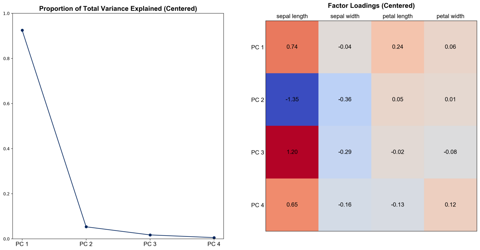
We can see that the first principal component explains over 90% of the total variance and it’s heavily dependent on sepal and petal length. This means that most of the variations in our data can be accounted for with a linear combination of these two features.
Using PCA as a dimensionality reduction or feature engineering tool will generally harm the interpretability of the results. When the number of features is much higher, each principal component is often a linear combination of too many distinct original features and hence hard to define.
To see the effect of standardization, transform the feature matrix so that each column has a standard deviation one and repeat the visualization.
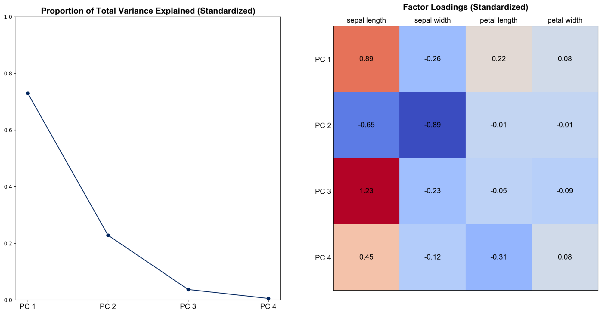
We can see that the results change quite much. Now the first principal component can only explain nearly 75% of the total variance, nearly 95% combined with the second. Sepal width becomes more important, especially for PC 2. Hence, there is no universal answer to the question of whether we should perform PCA on the covariance or the correlation matrix. The “best” method is based on a subjective choice, careful thought, and some experience.
This blog was originally published on @Medium with @Towards Data Science at this link.
Background picture source: Lars_Nissen on Pixabay
-
Previous
Multicollinearity and Ridge Regression -
Next
Estimate Population Variance: should we divide by n - 1 or n