This article discusses what is multicollinearity, how can it compromise least squares, and how ridge regression helps avoid that from a perspective of singular value decomposition (SVD). It is heavily based on Professor Rebecca Willet’s course Mathematical Foundations of Machine Learning and it assumes basic knowledge of linear algebra.
Multicollinearity
Consider a matrix $X$ of shape $n × p$. For its columns $X_1, X_2, \dots, X_p \in \mathbb{ℝ}^n$, we say they are linearly independent when $\sum{\alpha_iX_i} = 0$ if and only if $\alpha_i = 0$ for $i = 1, 2, \dots, p$. Intuitively, none of the columns in $X$ can be written as a weighted sum of the others. The other way around, if it’s not the case for some columns, we call them linearly dependent. Assume $\operatorname{rank}(X)=p$, then $(p-r)$ columns of X are linearly dependent.
Multicollinearity, in regression terms, refers to a phenomenon where a predictor in a multiple regression model can be linearly predicted from the others with a substantial degree of accuracy. In other words, the predictor is approximately a linear combination of the others. Perfect multicollinearity indicates linear dependency in the feature matrix. Intuitively, it implies redundancy in our features that some of them fail to provide unique and/or independent information to the regression.
Multicollinearity matters not only theoretically, but also for the practice. The coefficient estimates may change erratically in response to small changes in the model or the data, and themselves do not make sense at all. Why is that? We’ll look at it from an SVD perspective. Before that, below is a quick recap on SVD.
Singular Value Decomposition
This section provides a basic introduction to SVD. Consider a matrix $X$ of shape $n \times p$. There always exists matrices $U$, $\Sigma$, $V$ such that $X=U_{n \times n} \Sigma_{n \times p} V_{p \times p}^{T}$. Both $U$ and $V$ are orthogonal ($U^{T} U=U U^{T}=I$, and $V^{T} V=V V^{T}=I$), and $Σ$ is diagonal.
The columns of $U$ are the left singular vectors, they form an orthonormal basis for the columns of $X$. The diagonal elements of $Σ$ are called singular values $\sigma_{1} \geq \sigma_{2} \geq \ldots \geq \sigma_{p} \ge 0$. The number of non-zero singular values is the rank of the matrix $X$, and the columns of Σ are the basis for the rows of $X$. The rows of $V$ are called the right singular vectors, they are the basis coefficients on the columns of $UΣ$ to represent each column of $X$.
Least Squares with Multicollinearity
Recall that for the feature matrix $X$ and the target variable $y$, least squares attempts to approximate the solution of the linear system $y=Xw$ by minimizing the sum of squares of the residuals $|y-X w|^{2}$. The weights vector $\hat{w}_\text{LS}$ can be written with the normal equation:
\begin{equation}\hat{w}_\text{LS}=\left(X^{T} X\right)^{-1} X^{T} y\end{equation}
Note that $X^TX$ is invertible if and only if $n\ge p$ and $\operatorname{rank}(X)=p$. Now it’s not hard to see why perfect multicollinearity is a major problem for least squares: it implies that the feature matrix is not full-rank so we cannot find a proper set of coefficients that minimize the sum of squared residuals.
However, why multicollinearity, or strong multicollinearity in specific, is problematic, either? Let’s find out from an SVD perspective.
Consider the true weights $w$, we know that $y = Xw + \epsilon$, where $\epsilon$ is some neglectable noise or error. We know that:
\begin{equation}\begin{aligned}\hat{w}_{\text{LS}}&=\left(X^{T} X\right)^{-1} X^{T} y=(X^{T}X)^{-1}X^T(Xw+\epsilon) \\ &=w+(X^TX)^{-1}X^T\epsilon\end{aligned}\end{equation}
We can see that the least squares coefficients deviate from the true weights by $\epsilon$ multiplied by some inflation term. Take a closer look at the inflation term $(X^TX)^{-1}X^T=V\Sigma^\dagger U^T$, where $X=U\Sigma V^T$, and $\Sigma^\dagger$ is the pseudo-inverse of $\Sigma$ and is of shape $p \times n$. We can get this by transposing $\Sigma$, and take the reciprocals of its diagonal elements.
If all the columns of X are linearly independent, we still have $p$ singular values and $\sigma_{1} \geq \sigma_{2} \geq \ldots \geq \sigma_{p} \ge 0$. However, with the presence of multicollinearity, some $\sigma_{i}$, $\sigma_{p}$ for example, will be close to zero. Then the diagonal element $\frac{1}{\sigma_{p}}$ will be huge, leading to a really large inflation term and therefore a great deviation in the least squares weights from the true weights.
Intuitively, multicollinearity can compromise least squares as it leads to small singular values. The estimation errors of the coefficients are inflated by the reciprocals of those singular values and therefore become too large to be neglected. How can we avoid this? One possibility is ridge regression.
Ridge Regression
Ridge regression builds on least squares by adding a regularization term in the cost function so that it becomes $|y-X w|^{2}+\lambda|w|^{2}$, where $\lambda$ indicates the strength of regularization.
We can write the cost function $L(w) = y^{T} y-2 w^{T} X^{T} y+w^{T} X^{T} X w+\lambda w^{T} w$. Then we can compute the gradient and set it to zero, $\nabla_{w} f=0-2 X^{T} y+2 X^{T} X w+2 \lambda w=0$. It solves to:
\begin{equation}\hat{w}_\text{R L S}=\left(X^{T} X+\lambda I\right)^{-1} X^{T} y=V\left(\Sigma^{T} \Sigma+\lambda I\right)^{-1} \Sigma^{T} U^{T} y\end{equation}
Take a closer look at $\left(\Sigma^{T} \Sigma+\lambda I\right)^{-1} \Sigma^{T}$, we can see it’s nothing but the transpose of $\Sigma$, while its diagonal elements are $\frac{\sigma_i}{\sigma_i^2+\lambda}$. How does this help?
Consider $σ_p \approx 0$, this time $\frac{\sigma_p}{\sigma_p^2+\lambda}\approx0$ if $λ \ne 0$. Therefore, with ridge regression, the coefficients of unimportant features will be close to zero (but will not be exactly 0 unless there is perfect multicollinearity) and the error term would not be inflated to an explosion. Note that when there is no regularization ($λ = 0$) things go back to least squares. Also, for most occasions where $σ_i \gg \lambda$, $\frac{\sigma_i}{\sigma_i^2+\lambda}$ behaves just like least squares.
Numerical Experiment
In this section, we’ll work on a sample dataset *seatpos* to verify our previous findings. The dataset is available at this link. It contains the following features:
We want to fit a linear model that predicts hipcenter based on all the other features in the dataset. From the descriptions, some features can be closely related to one another. For example, Weight and Ht, Ht and HtShoes. Plot the correlation matrix:
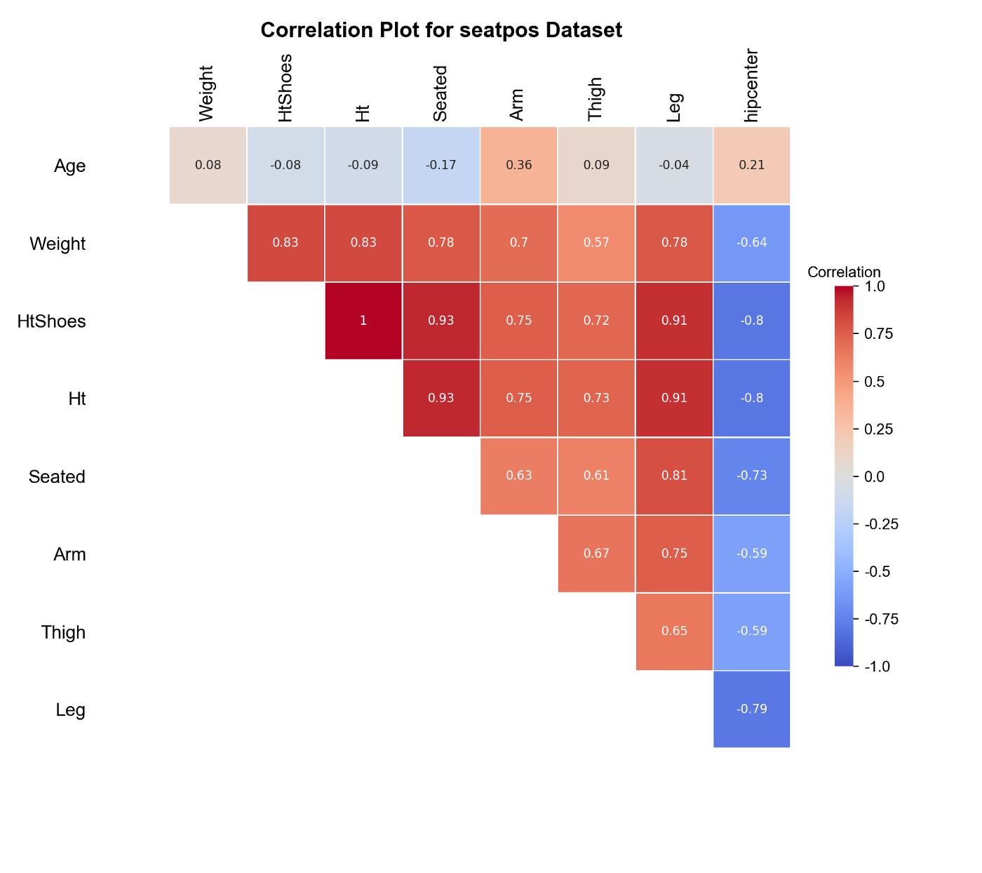
The plot above confirms our guess. We have strong multicollinearity in our feature matrix. The good news is that our target hipcenter is strongly correlated with most of the features and we can expect a good fit.
Use the following code chunk to:
- Add an offset to the feature matrix
- Split the dataset into training and test set
- Normalize the feature matrix so that we can compare the coefficients, as we expect features with larger variations to have smaller coefficients, ceteris paribus
For simplicity, first look at a model with only Ht and HtShoes as predictors.
1
2
3
4
5
6
7
X_train_sub = X_train_[:, 2:4]
X_test_sub = X_test_[:, 2:4]
ls = LinearRegression(fit_intercept=True)
ls.fit(X_train_sub, y_train)
print(ls.intercept_, ls.coef_)

# Output: -165.844 [54.745 -105.923]
Surprisingly, although Ht and HtShoes are nearly perfectly correlated, their partial effects on hipcenter have the opposite signs. This can be a result of strong multicollinearity. Fit a ridge regression model with λ = 10 instead.
1
2
3
4
5
ridge = Ridge(alpha=10)
ridge.fit(X_train_sub, y_train)
print(ridge.intercept_, ridge.coef_)

# Output: -165.844 [-21.593  -22.269]
The coefficients of ridge regression seem to make more sense. Compare its test RMSE with that of the least squares.
1
2
3
4
5
6
7
8
ls_rmse = mean_squared_error(y_test, ls.predict(X_test_sub))
ridge_rmse = mean_squared_error(y_test, ridge.predict(X_test_sub))

print(f"Least squares test RMSE: {ls_rmse:.3f}")
print(f"Ridge test RMSE: {ridge_rmse:.3f}")

# Least squares test RMSE: 643.260
# Ridge test RMSE: 519.287
For the bivariate linear model, ridge regression results in a better ability to generalize. However, since ridge regression introduces a regularization term, its bias can be higher in exchange for a lower variance sometimes, which may lead to worse fit.
At last, let’s look at the full model and check how the magnitudes of the coefficients differ across least squares and ridge regression, and how they change with the strength of penalty, $\lambda$.
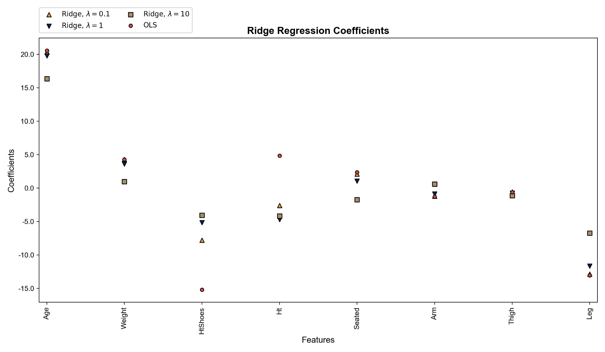
We can see that least squares weights differ greatly from ridge regression weights on Ht and HtShoes as expected. Ridge regression weights get closer to zero as the penalty gets stronger. Codes that produces the plot above:
This blog was originally published on @Medium with @Towards Data Science at this link.