This blog discusses the difference in least-squares weight vectors across over- and underdetermined linear systems, and how singular value decomposition (SVD) can be applied to derive a consistent expression. It is heavily based on Professor Rebecca Willet’s course Mathematical Foundations of Machine Learning and it assumes basic knowledge of linear algebra.
Typical Least Squares
Least squares can be described as follows: given the feature matrix $X$ of shape $n \times p$ and the target vector $y$ of shape $n \times 1$, we want to find a coefficient vector $\hat{w}$ of shape $n \times 1$ that satisfies $\hat{w} = \operatorname{argmin}{|y-X w|^{2}}$. Intuitively, least squares attempts to approximate the solution of linear systems by minimizing the sum of squares of the residuals made in the results of every single equation.
On most occasions, we assume that $n \ge p$ and $\operatorname{rank}(X)=p$. In other words, the number of observations is no less than that of features and none of the features is a linear combination of the others (no “redundant” features). A linear system $y = Xw$ is overdetermined if $n \ge p$. We can get $\hat{w}$ with the normal equation:
\begin{equation}\hat{w}=\left(X^{T} X\right)^{-1} X^{T} y\end{equation}
However, if $n < p$ or when some columns in $X$ are linearly dependent, the matrix $X^TX$ may not be invertible. When the number of features is larger than that of observations, we call the linear system $y = Xw$ underdetermined.
Underdetermined Least Squares
When $n < p$ and ,$\operatorname{rank}(X)=n$ there are infinitely many solutions to the system $y = Xw$. Among these solutions, we can find the one with the smallest norm via the method of Lagrange multiplier and use it as the least-squares weight vector for the underdetermined linear system.
However, why is the least-norm solution desirable? One hand-wavy way to look at this: the third feature is small in scale. If it’s vulnerable to measurement error and we assign a large weight to it, our predictions on unseen data can be heavily biased by the third feature alone and thus far from the true target. Therefore, the first solution is better.
we want to minimize $|w|^{2}$ with the constraint that $y = Xw$. Introduce the Lagrange multiplier $L(w, \lambda)=w^{T} w+\lambda^{T}(X w-y)$. Under the optimal conditions that $\nabla_{w} L=2 w+X^{T} \lambda=0$, $\nabla_{\lambda} L=X w-y=0$, we have:
\begin{equation}\hat{w}=X^{T}\left(X X^{T}\right)^{-1} y\end{equation}
The equation of the weight vector for underdetermined least squares is very different from that for overdetermined least squares.
Singular Value Decomposition
This section provides a basic introduction to SVD. Consider a matrix $X$ of shape $n \times p$. There always exists matrices $U$, $\Sigma$, $V$ such that $X=U_{n \times n} \Sigma_{n \times p} V_{p \times p}^{T}$. Where both $U$ and $V$ are orthogonal ($U^{T} U=U U^{T}=I$, and $V^{T} V=V V^{T}=I$), and $Σ$ is diagonal.
The columns of $U$ are the left singular vectors, they form an orthonormal basis for the columns of $X$. The diagonal elements of $Σ$ are called singular values $\sigma_{1} \geq \sigma_{2} \geq \ldots \geq \sigma_{p} \ge 0$. The number of non-zero singular values is the rank of the matrix $X$, and the columns of Σ are the basis for the rows of $X$. The rows of $V$ are called the right singular vectors, they are the basis coefficients on the columns of $UΣ$ to represent each column of $X$.
SVD and Least Squares
With SVD, we can rewrite the least-squares weight vectors. Use that of the underdetermined least squares as an example:
\begin{equation}X^{T}\left(X X^{T}\right)^{-1}=V \Sigma^{T} U^{T}\left(U \Sigma V^{T} V \Sigma^{T} U^{T}\right)^{-1}=V \Sigma^{T}\left(\Sigma \Sigma^{T}\right)^{-1} U^{T}\end{equation}
The expression above can seem a bit daunting, but if we take a closer look: $\Sigma^{T}\left(\Sigma \Sigma^{T}\right)^{-1}=\Sigma^{\dagger}$. Here $\Sigma^\dagger$ is the pseudo-inverse of $\Sigma$ and is of shape $p \times n$. We can get this by transposing $\Sigma$, and take the reciprocals of its diagonal elements. Then the least-squares vector of an underdetermined linear system can be rewritten as:
\begin{equation}\hat{w}=X^{T}\left(X X^{T}\right)^{-1} y=V \Sigma^{\dagger} U^{T} y\end{equation}
Numerical Experiment
To verify our findings, we will use a subsample of the Jester Datasets. The sample contains 100 observations and 7200 features and it is available here. Each observation is a joke and each feature is a known rating on that joke from an existing user, at a scale of -10 to 10.
Suppose that we work for a company that makes joke recommendations to customers based on their known ratings. For a new customer Joan who has rated 25 jokes, we want to be able to know how she would like the remaining 75 jokes and recommend her the one with the highest predicted rating.
To do that, consider $m$ ($m \le 7200$) users whose ratings on the 100 jokes are known to us. They represent a diverse set of tastes. We can think of Joan’s ratings as a weighted sum of these customers’ ratings. Then, we will use the 25 joke ratings by these $m$ customers as features and Joan’s known ratings as the target to train a regressor. It should be able to generalize to other jokes that Joan hasn’t rated yet with good predictions so that we can recommend the one with the highest predicted score. Joan’s ratings are available here.
Load data and split it into training and test set with the following chunk. Note that Joan’s unknown ratings are represented as -99.
When $m = 20$, we would use the first 20 users as our representative users for simplicity. We will solve for the weights with their ratings on the 25 jokes that Joan has rated as features and Joan’s ratings as the target. The linear system is overdetermined. When $m = 7200$, the linear system is underdetermined. Use the following codes to prepare the data.
A scikit-learn style least-squares estimator using SVD is implemented as follows:
I got True for both $m = 20$ and $m = 7200$. Feel free to verify it yourself.
To illustrate how underdetermined least squares provides a perfect fit to the training data, we can visualize the predicted values and the true target on both training and test sets.
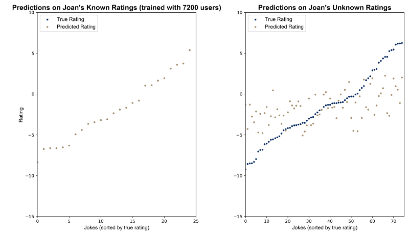
Corresponding codes is available below.
This blog was originally published on @Medium with @Towards Data Science at this link.